Plot recipes

Some recipes are available to visualize computed problems solution. You need to import the package Plots.jl.

Surface deformation and velocity

using Plots

param = ( μ = 1, ϵ = 1/4, N = 2^10, L = 10, T = 5, dt = 0.01 )
z(x) = exp.(-abs.(x).^4)
v(x) = zero(x)
init = Init(z,v)

model0 = WaterWaves(param; tol = 1e-15)  # The water waves system
model1 = Airy(param)                     # The linear model (Airy)
model2 = WWn(param;n=2,dealias=1,δ=1/10) # The quadratic model (WW2)

problem0 = Problem(model0, init, param);
problem1 = Problem(model1, init, param);
problem2 = Problem(model2, init, param);

solve!([problem0 problem1 problem2]; verbose=false);


plot(problem0)
plot!(problem1)
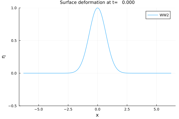
plot!(problem2; var = :surface, legend = :bottomright)

plot([problem0, problem1, problem2]; var = :velocity, legend = :bottomright)

Differences

plot([problem0, problem1], var = :difference)
plot!([problem0, problem2], var = :difference)

plot([(problem0, problem1), (problem0, problem2)])

plot([(problem0, problem1), (problem0, problem2)], var = :difference_velocity)

Fourier coefficients

using Plots

η(x) = exp.(-x.^2)
v(x) = zero(x)
init = Init(η,v)

param1 = ( ϵ = 1/4, μ = Inf, N = 2^8, L = 2*π, T = 5, dt = 0.001 )

problem1 = Problem( WWn(param1, dealias = 1), init, param1 )

param2 = ( ϵ = 1/4, μ = Inf, N = 2^9, L = 2*π, T = 5, dt = 0.001 )

problem2 = Problem( WWn(param2, dealias = 1), init, param2 )

solve!([problem1, problem2])

plot([problem1, problem2]; T=5, var = :fourier)

Subplots

l = @layout [a ; b; c]
p1 = plot(problem1, var = :surface)
p2 = plot(problem1, var = :velocity)
p3 = plot(problem1, var = :fourier)
plot(p1, p2, p3, layout = l,
	 titlefontsize=10,
	 labelfontsize=8)

plot(problem1, var = [:surface,:velocity,:fourier])

Interpolation

x̃ = LinRange(-5, 5, 128)
plot(problem2, x = x̃, shape = :circle)

Plots at different times

plot(problem1, T = 0, label = "t = 0")
for t in 1:5
    plot!(problem1, T = t, label = "t = $t")
end
title!("surface deformation for t ∈ [0,5]")

Create animation

@gif for t in LinRange(0,param1.T,100)
    plot(problem1, T = t)
    ylims!(-0.5, 1)
end