Hammack-Segur

This notebook provides a comparison of several models for water waves on the results of an experiment of Hammack & Segur experiment, in the spirit of Carter.

Initialization

Import package

using WaterWaves1D

Define parameters of the problem

d = 0.1;  # depth of the basin (in m)g = 9.81; # gravitational accelerationλ = 0.1;  # typical horizontal length (=d to simplify)T = 40;   # final time (in s)L = 156.16; # half-length of the numerical tank (in m)param = (    # Physical parameters. Variables are non-dimensionalized as in Lannes, The water waves problem, isbn:978-0-8218-9470-5    μ = 1,    # shallow-water dimensionless parameter    ϵ = 1,    # nonlinearity dimensionless parameter    # Numerical parameters    N = 2^12, # number of collocation points    L = L / d,       # half-length of the numerical tank ( = 156.16 m)    T = T * sqrt(g * d) / λ, # final time of computation (= 50 s)    dt = T * sqrt(g * d) / λ / 10^3, # timestep)

(μ = 1, ϵ = 1, N = 4096, L = 1561.6, T = 396.18177646126026, dt = 0.39618177646126024)

Define initial data (as in Carter).

using Elliptic, Plotsa = 0.005 # half-amplitude of the initial data (in m)sn(x) = getindex.(ellipj.(9.25434 * x * d, 0.9999^2), 1);  # regularized step functionη0(x) = (-1 / 2 * a .+ 1 / 2 * a * sn(x)) .* (x * d .< 0.61) .* (x * d .> -1.83) / d;init = Init(x -> 2 * η0(x), x -> zero(x));         # generate the initial data with correct typex = Mesh(param).xplot(    x, [init.η(x) * d init.v(x)],    title = "initial data",    label = ["surface deformation" "velocity"],    xlims = (-20, 10))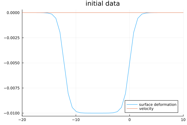

Set up initial-value problems for different models to compare

model_WW2 = WWn(param; n = 2, dealias = 1, δ = 1 / 10) # The quadratic water waves model (WW2)model_SGN = SerreGreenNaghdi(param) # The Serre-Green-Naghdi model (SGN)model_WGN = WhithamGreenNaghdi(param) # The fully dispersive Whitham-Green-Naghdi model (WGN)

Whitham-Green-Naghdi model.
├─Shallowness parameter μ=1, nonlinearity parameter ϵ=1.
├─No dealiasing. No Krasny filter. 
└─Elliptic problem solved with GMRES method with preconditioning, tolerance 1.0e-14, maximal number of iterations 4096, restart after 20 iterations (consider `iterate=false` for non-iterative method). 
Discretized with 4096 collocation points on [-1561.6, 1561.6].

type ?WaterWaves or ?WWn, etc. to see details and signification of arguments

WW2 = Problem(model_WW2, init, param) ;SGN = Problem(model_SGN, init, param) ;WGN = Problem(model_WGN, init, param) ;

Computation

Solve integration in time

solve!(WW2);solve!(SGN);solve!(WGN);

┌ Info: Now solving the initial-value problem WW2
│ with timestep dt=0.39618177646126024, final time T=396.18177646126026,
└ and N=4096 collocation points.

┌ Info: Now solving the initial-value problem Green-Naghdi
│ with timestep dt=0.39618177646126024, final time T=396.18177646126026,
└ and N=4096 collocation points.

┌ Info: Now solving the initial-value problem Whitham-Green-Naghdi
│ with timestep dt=0.39618177646126024, final time T=396.18177646126026,
└ and N=4096 collocation points.

Visualization

Import the data (from the Hammack\&Segur experiment, kindly provided by Carter)

using DelimitedFilesdata_dir = joinpath(pkgdir(WaterWaves1D), "examples", "data");data2a = readdlm(joinpath(data_dir, "Fig2aFixed.out"), '\t');data2b = readdlm(joinpath(data_dir, "Fig2bFixed.out"), '\t');data2c = readdlm(joinpath(data_dir, "Fig2cFixed.out"), '\t');data2d = readdlm(joinpath(data_dir, "Fig2dFixed.out"), '\t');data2e = readdlm(joinpath(data_dir, "Fig2eFixed.out"), '\t');"""    gauge(p::Problem;x,t)Give the surface elevation provided by a problemat a specific location `x` (by default, `x=0`),and at times defined by `t` if provided (otherwise at all computed times)."""function gauge(p::Problem; x = 0, T = nothing)    if T == nothing        times = p.times.ts    elseif T[1] == T        times = [T]    else        times = T    end    return times / sqrt(g * d) * λ, [solution(p, T = ti, x = [x])[1][1] for ti in times] * dend

Plot data and numerics at first gauge

plt = plot(    data2a[:, 1] / sqrt(g * d) * λ, data2a[:, 2] * d * 2 / 3,    title = "first gauge",    label = "experiment",    xlabel = "time (in s)",    ylabel = "surface deformation (in m)")plot!(    [gauge(WW2, x = 1), gauge(SGN, x = 1), gauge(WGN, x = 1)],    label = ["WW2" "SGN" "WGN"])xlims!(0, 5)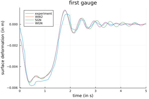

Plot data and numerics at second gauge

plt = plot(    (data2b[:, 1] .+ 50) / sqrt(g * d) * λ, data2b[:, 2] * d * 2 / 3,    title = "second gauge",    label = "experiment",    xlabel = "time (in s)",    ylabel = "surface deformation (in m)")plot!(    [gauge(WW2, x = 51), gauge(SGN, x = 51), gauge(WGN, x = 51)],    label = ["WW2" "SGN" "WGN"])xlims!(5, 17)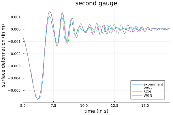

Plot data and numerics at third gauge

plt = plot(    (data2c[:, 1] .+ 100) / sqrt(g * d) * λ, data2c[:, 2] * d * 2 / 3,    title = "third gauge",    label = "experiment",    xlabel = "time (in s)",    ylabel = "surface deformation (in m)")plot!(    [gauge(WW2, x = 101), gauge(SGN, x = 101), gauge(WGN, x = 101)],    label = ["WW2" "SGN" "WGN"])xlims!(10, 30)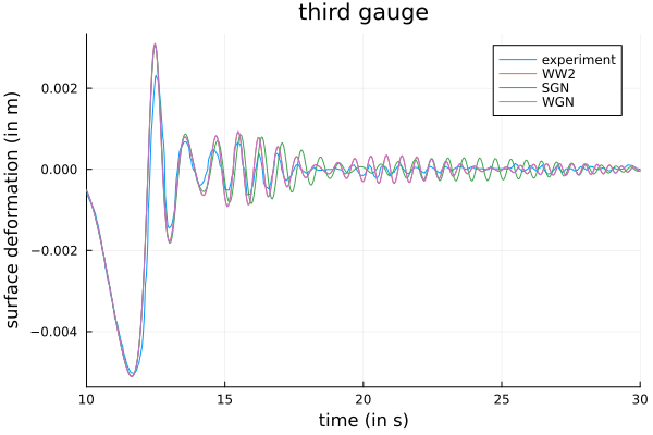

Plot data and numerics at fourth gauge

plt = plot(    (data2d[:, 1] .+ 150) / sqrt(g * d) * λ, data2d[:, 2] * d * 2 / 3,    title = "fourth gauge",    label = "experiment",    xlabel = "time",    ylabel = "surface deformation")plot!(    [gauge(WW2, x = 151), gauge(SGN, x = 151), gauge(WGN, x = 151)],    label = ["WW2" "SGN" "WGN"])xlims!(15, 35)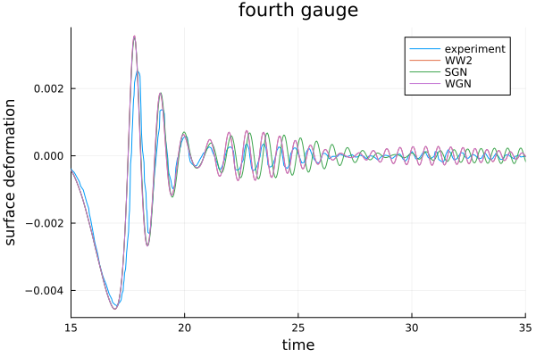

Plot data and numerics at fifth gauge

plt = plot(    (data2e[:, 1] .+ 200) / sqrt(g * d) * λ, data2e[:, 2] * d * 2 / 3,    title = "fifth gauge",    label = "experiment",    xlabel = "time",    ylabel = "surface deformation")plot!(    [gauge(WW2, x = 201), gauge(SGN, x = 201), gauge(WGN, x = 201)],    label = ["WW2" "SGN" "WGN"])xlims!(20, 40)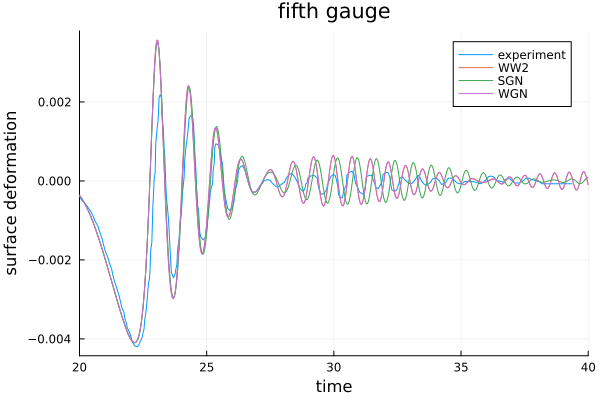

The quadratic water waves model and Whitham-Green-Naghdi model predict are almost indistinguishable, because the steepness of the wave is very small.

This page was generated using Literate.jl.