Quick Start Example

In this example we shall observe the disintegration of a heap of water using the water-waves system as well as a second-order small-steepness model.

More advanced examples can be found in the package's examples folder. Examples are also available through the functions examples_dir, get_examples and default_example.

Set up the initial-value problem

First we define parameters of our problem.

using WaterWaves1Dparam = (    # Physical parameters. Variables are non-dimensionalized as in Lannes,    # The water waves problem, isbn:978-0-8218-9470-5    μ = 1,     # shallow-water dimensionless parameter    ϵ = 1 / 4,   # nonlinearity dimensionless parameter    # Numerical parameters    N = 2^10,  # number of collocation points    L = 10,    # half-length of the numerical tank (-L,L)    T = 5,     # final time of computation    dt = 0.01,  # timestep)

(μ = 1, ϵ = 0.25, N = 1024, L = 10, T = 5, dt = 0.01)

Now we define initial data solver (the "heap of water"). The function Init may take either functions, or vectors (values at collocation points) as arguments.

z(x) = exp.(-abs.(x) .^ 4); # surface deformationv(x) = zero(x);     # zero initial velocityinit = Init(z, v);         # generate the initial data with correct type

Then we build the different models to compare (see WaterWaves and WWn).

model_WW = WaterWaves(param) # The water waves systemmodel_WW2 = WWn(param; n = 2, dealias = 1, δ = 1 / 10) # The quadratic model (WW2)

Spectral model of order 2.
├─Shallowness parameter μ=1, nonlinearity parameter ϵ=0.25, scaling parameter ν=1 (shallow water case).
├─Rectifier with strength δ=0.1 and order m=-1.
└─Dealiasing with Orszag's rule adapted to power 2 nonlinearity. No Krasny filter. 
Discretized with 1024 collocation points on [-10.0, 10.0].

Finally we set up initial-value problems. Optionally, one may specify a time solver to Problem (by default the standard explicit fourth order Runge Kutta method is used).

problem_WW = Problem(model_WW, init, param)problem_WW2 = Problem(model_WW2, init, param)

Initial-value problem with...
├─Model: WW2.
├─Initial data: user-defined.
├─Solver: RK4.
└─Grid of times: 501 computed times on [0, 5.0] (timestep dt=0.01), among which 501 will be stored.

Solve the initial-value problem

Solving the initial-value problems is as easy as solve!.

solve!([problem_WW problem_WW2]; verbose = false);

Evaluate the precision of the numerical scheme

The numerical discretization of preserved quantities, provided by the functions mass, momentum, energy (and mass_diff, momentum_diff, energy_diff for the difference between initial and final time) provide valuable insights at the precision of a computed numerical solution.

Δ = [mass_diff(problem_WW2), momentum_diff(problem_WW2), energy_diff(problem_WW2)]

3-element Vector{Float64}:
  4.6214117602194626e-17
  2.8762000476657894e-19
 -6.633679716649965e-11

Generate graphics

Plot solutions at final time.

using Plotsplot([problem_WW, problem_WW2])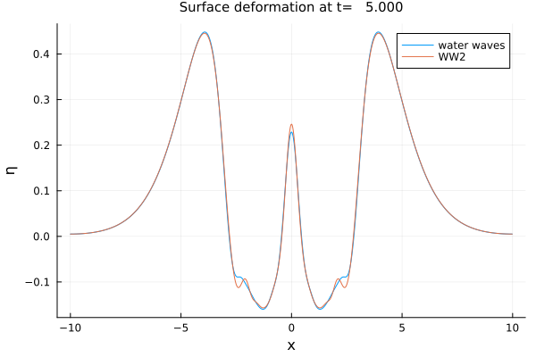

Generate an animation.

@gif for t in LinRange(0, param.T, 100)    plot([problem_WW, problem_WW2], T = t)    ylims!(-0.5, 1)end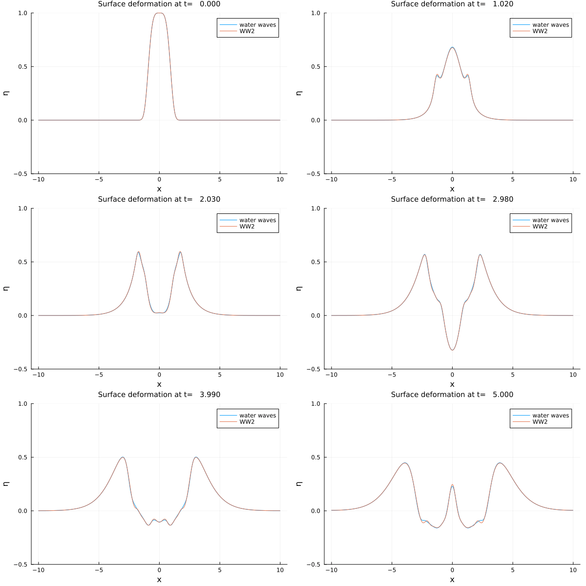

See the plot recipes for many more plotting possibilities.

This page was generated using Literate.jl.