Shallow-Water

In this notebook, we provide a comparison of several non-hydrostatic shallow-water models for the propagation of surface gravity waves. Specifically, we compare the standard Green-Naghdi model

first with the non-hydrostatic model of Bristeau, Mangeney, Sainte-Marie and Seguin and the square-root depth system of Cotter, Holm and Percival,
then with the fully dispersive counterpart of Duchêne, Israwi and Talhouk,
finally with the Isobe-Kakinuma model.

Initialization

Import package

using WaterWaves1Dimport LinearAlgebra.norm

Define parameters of the problem

param = (    # Physical parameters. Variables are non-dimensionalized as in Lannes, The water waves problem, isbn:978-0-8218-9470-5    μ = 0.1,   # shallow-water dimensionless parameter    ϵ = 0.25,   # nonlinearity dimensionless parameter    # Numerical parameters    N = 2^9,  # number of collocation points    L = π,    # half-length of the numerical tank (-L,L)    T = 1,    # final time of computation    dt = 0.01, # timestep);

Define initial data

random = Random(param; L = 1);     # randomly generate initial data. Type `?random` for possible parameterization.init = Init(random.η, zero); # we set the initial velocity as zero to avoid inconsistencies among different models.using Plotsx = Mesh(param).xplot(x, [init.η(x) init.v(x)], label = ["surface deformation" "velocity"], title = "Initial data")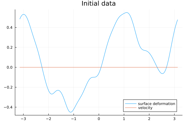

First-order non-hydrostatic models

Here we shall compare the Green-Naghdi model with the non-hydrostatic model of Bristeau, Mangeney, Sainte-Marie and Seguin and the square-root depth system of Cotter, Holm and Percival

Set up initial-value problems for different models to compare

WW = Problem(WaterWaves(param, dealias = 1, verbose = false), init, param)GN = Problem(SerreGreenNaghdi(param; dealias = 0, iterate = true, precond = true), init, param)NH = Problem(NonHydrostatic(param; dealias = 0, iterate = true, precond = true), init, param)SRD = Problem(SquareRootDepth(param; dealias = 0, iterate = true, precond = true), init, param)solve!(WW);solve!(GN);solve!(NH);solve!(SRD);

┌ Info: Now solving the initial-value problem water waves
│ with timestep dt=0.01, final time T=1.0,
└ and N=512 collocation points.

┌ Info: Now solving the initial-value problem Green-Naghdi
│ with timestep dt=0.01, final time T=1.0,
└ and N=512 collocation points.

┌ Info: Now solving the initial-value problem non-hydrostatic
│ with timestep dt=0.01, final time T=1.0,
└ and N=512 collocation points.

┌ Info: Now solving the initial-value problem square-root depth
│ with timestep dt=0.01, final time T=1.0,
└ and N=512 collocation points.

Plot solutions at final time

plot([WW, GN, SRD, NH])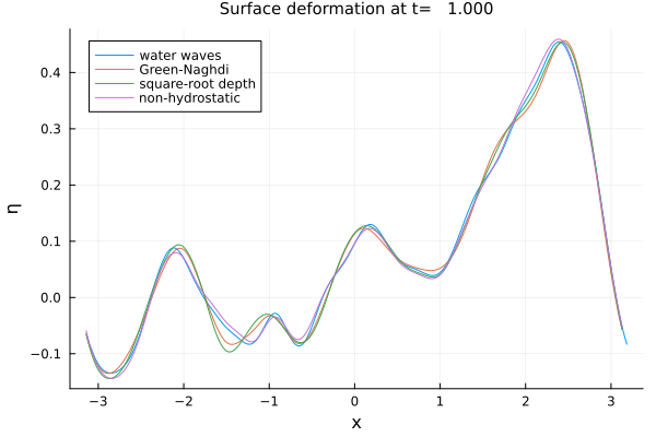

plt = plot([(WW, GN), (WW, SRD), (WW, NH)])display(plt)

WWη, WWv, WWx, = solution(WW)GNη, = solution(GN, x = WWx);errGN = norm(WWη - GNη) / sqrt(length(x))SRDη, = solution(SRD, x = WWx);errSRD = norm(WWη - SRDη) / sqrt(length(x))NHη, = solution(NH, x = WWx);errNH = norm(WWη - NHη) / sqrt(length(x))print("Errors (in l²). Serre-Green-Naghdi: $errGN, Square-root depth: $errSRD, Non-hydrostatic: $errNH")

Errors (in l²). Serre-Green-Naghdi: 0.009900811970557817, Square-root depth: 0.009522380103608395, Non-hydrostatic: 0.006757434147535756

Using the notation and terminology of Lannes, The water waves problem (isbn:978-0-8218-9470-5),

the Green-Naghdi model is consistent with precision O(μ²)
the Square-root-depth model is consistent with precision O(μ²+μϵ)
the Non-hydrostatic model is consistent with precision O(μ)

This can be checked by varying the parameters μ,ϵ

It happens however quite often when μ is fairly large (or L in the random initial data is small) that the non-hydrostatic model provides a better approximation than the Green-Naghdi and square-root-depth model. A possible explanation stems from the fact that the wave frequency of the former (ω(k)=±|k|(1/(1+¼μ|k|^2))^½) approaches better the wave frequency of the water waves system (ω(k)=±|k|(tanh(√μ|k|)/(√μ|k|))^½) for a finite range of wavenumbers, k, while the group velocity of the latter (ω(k)=±|k|(1/(1+⅓μ|k|^2))^½) is more accurate only for small wavenumbers.

Fully dispersive model

Here we shall compare the Green-Naghdi model with the fully dispersive counterpart of Duchêne, Israwi and Talhouk.

Set up initial-value problems for different models to compare

WW = Problem(WaterWaves(param, dealias = 1, verbose = false), init, param)GN = Problem(SerreGreenNaghdi(param; dealias = 0, iterate = true, precond = true), init, param)WGN = Problem(WhithamGreenNaghdi(param; dealias = 0, iterate = true, precond = true), init, param)solve!(WW);solve!(GN);solve!(WGN);

┌ Info: Now solving the initial-value problem water waves
│ with timestep dt=0.01, final time T=1.0,
└ and N=512 collocation points.

┌ Info: Now solving the initial-value problem Green-Naghdi
│ with timestep dt=0.01, final time T=1.0,
└ and N=512 collocation points.

┌ Info: Now solving the initial-value problem Whitham-Green-Naghdi
│ with timestep dt=0.01, final time T=1.0,
└ and N=512 collocation points.

Plot solutions at final time

plot([WW, GN, WGN])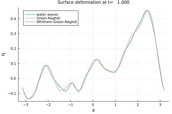

plt = plot([(WW, GN), (WW, WGN)])display(plt)

WWη, WWv, WWx, = solution(WW)GNη, = solution(GN, x = WWx);errGN = norm(WWη - GNη) / sqrt(length(x))WGNη, = solution(WGN, x = WWx);errWGN = norm(WWη - WGNη) / sqrt(length(x))print("Errors (in l²). Serre-Green-Naghdi: $errGN, Whitham-Green-Naghdi: $errWGN")

Errors (in l²). Serre-Green-Naghdi: 0.009900811970557817, Whitham-Green-Naghdi: 0.0008347952799861205

Using the notation and terminology of Lannes, The water waves problem (isbn:978-0-8218-9470-5),

the Green-Naghdi model is consistent with precision O(μ²)
the fully dispersive model is consistent with precision O(μ²ϵ)

This can be checked by varying the parameters μ,ϵ

Higher-order model

Here we shall compare the Green-Naghdi model with the 2nd order Isobe-Kakinuma model.

Set up initial-value problems for different models to compare

WW = Problem(WaterWaves(param, dealias = 1, verbose = false), init, param)GN = Problem(SerreGreenNaghdi(param; dealias = 0, iterate = true, precond = true), init, param)IK = Problem(IsobeKakinuma(param; dealias = 0, iterate = true, precond = true), init, param)solve!(WW);solve!(GN);solve!(IK);

┌ Info: Now solving the initial-value problem water waves
│ with timestep dt=0.01, final time T=1.0,
└ and N=512 collocation points.

┌ Info: Now solving the initial-value problem Green-Naghdi
│ with timestep dt=0.01, final time T=1.0,
└ and N=512 collocation points.

┌ Info: Now solving the initial-value problem Isobe-Kakinuma
│ with timestep dt=0.01, final time T=1.0,
└ and N=512 collocation points.

Plot solutions at final time

plot([WW, GN, IK])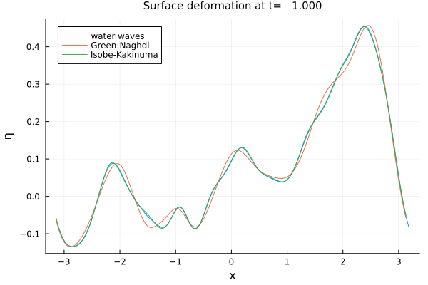

plt = plot([(WW, GN), (WW, IK)]; fourier = false)display(plt)

WWη, WWv, WWx, = solution(WW)GNη, = solution(GN, x = WWx);errGN = norm(WWη - GNη) / sqrt(length(x))IKη, = solution(IK, x = WWx);errIK = norm(WWη - IKη) / sqrt(length(x))print("Errors (in l²). Serre-Green-Naghdi: $errGN, Isobe-Kakinuma: $errIK")

Errors (in l²). Serre-Green-Naghdi: 0.009900811970557817, Isobe-Kakinuma: 0.0017109497755251387

Using the notation and terminology of Lannes, The water waves problem (isbn:978-0-8218-9470-5),

the Green-Naghdi model is consistent with precision O(μ²)
the Isobe-Kakinuma model is consistent with precision O(μ³)

This can be checked by varying the parameters μ,ϵ

Dispersion relations

We compare the dispersion relations of the models appearing in this notebook. Recall variables are non-dimensionalized. For instance, the real dispersion relation of the water waves system (linearized about the rest state) is ω(ξ)² = g|ξ| tanh(d|ξ|), where g is the gravity acceleration and d the depth of the layer.

k = abs.(Mesh(param).k);μ = param.μωWW(k) = k .* (tanh.(√μ * k) ./ (√μ * k)) .^ (1 / 2)ωNH(k) = k .* (1 ./ (1 .+ μ / 4 * k .^ 2)) .^ (1 / 2)ωGN(k) = k .* (1 ./ (1 .+ μ / 3 * k .^ 2)) .^ (1 / 2)ωIK(k) = k .* ((1 .+ μ / 15 * k .^ 2) ./ (1 .+ 2 * μ / 5 * k .^ 2)) .^ (1 / 2)plot(    k, [ωWW(k) ./ k ωGN(k) ./ k ωNH(k) ./ k ωIK(k) ./ k],    label = ["water waves and fully dispersive" "Green-Naghdi and square-root-depth" "Non-hydrostatic" "Isobe-Kakinuma"],    xlabel = "wavenumbers, k", ylabel = "phase velocity, ω(k)/k",    title = "dispersion relation")xlims!(0, 5 / μ)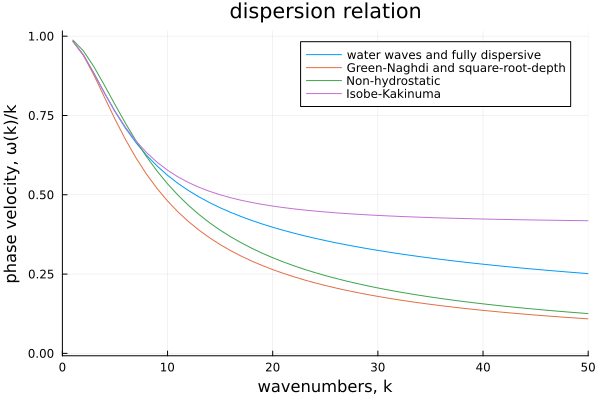

This page was generated using Literate.jl.